Single Transmission Line

When you wish to determine the transmission line parameters, Z0 and Eeff, for a single transmission line, you should use a standard box-wall port for the best results. It is not recommended that you use an ABS sweep, since the Z0 and Eeff data is only calculated for the discrete data points, but not for any adaptive data; therefore an analysis will yield very few data points. If there are any problems in calculating Z0 and Eeff, then em outputs an error message in place of a value.

Creating the Plot

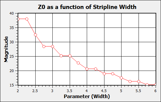
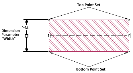
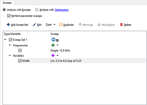
It is possible to plot Z0 or Eeff as a function of line width for a single transmission line by using a dimension parameter for the width of the feedline. You then analyze the circuit using a parameter sweep varying the width of the line over the desired range of values. Once you have the analysis results, you can use the response viewer to create a plot of your data. A detailed example is provided below.

This example uses a simple stripline circuit show below.

1.  Add a dimension parameter to vary the line width.
   
   A symmetric dimension parameter would work best with this circuit since it uses symmetry. The circuit is shown below with a symmetric dimension parameter “Width” added with its point sets highlighted. For more information about symmetric parameters and how to add them to your circuit, please see Insert ⇒ Dimension Parameter ⇒ Symmetric.

 .

2.  Set up a parameter sweep using the variable “Width.”
   
   For this example, the circuit will be analyzed using a parameter sweep, varying the width of the line from 2 mm to 6 mm in 0.25 mm increments at a single frequency of 15 GHz. The Parameter Sweep Entry dialog box for the analysis is shown below.
   
   
3.  Run the analysis, then open the response viewer.
   
   The response viewer may be opened by clicking on the Graph icon in the job queue tab (shown below) or selecting Launch - Graph Response from the main menu of the project editor tab or the job queue tab once the analysis has completed.

4.  Select Graph ⇒ Plot Over ⇒ Parameter from the main menu of the Response Viewer.

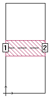
This will plot the selected data as a function of the value Width. If there were more than one parameter in your circuit, you would have had to choose which to use but since this circuit contains only one parameter, Width is automatically selected. The default measurement of S11 is plotted.

5. Select Graph ⇒ Manage Curves from the main menu of the response viewer. 

The Manage Curves dialog box appears on your display. The default curve of S11 is already selected in the Curves list since it is the only curve presently in your plot.

6.  Select “Line Z0” under Transmission Lines in the Measurement panel.

This will plot the characteristic impedance of the feedline connected to the selected port. The Properties panel is updated with the properties of the Input Impedance measurement. For this example, we will plot the Input Impedance for Port 1, so no change needs to be made to the properties. If there were more than one frequency available, you would have needed to click on the Parameters field and selected the frequencies you wish to plot

7.  Click on the Close button to close the Manage Curves dialog box.

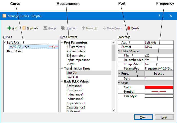
The plot shows the magnitude of the characteristic impedance of Port 1 as a function of line width. The characteristic impedance goes down as the line gets wider. If you wished to plot the Eeff, you would have chosen “Line Eeff” from the Measurement list.